Image Stitching: Part 1
This is Part 1 of 2 in my posts about how to stitch two images together using Julia. It’s rough around the edges, since I’m learning how to do this myself. In Part 1 I talk about finding keypoints, descriptors, and matching two images together. Next time, I’ll talk about how to estimate the image transformation and how to actually do the stitching.
I’ve included my notebook here. You can see the original on Github if you like.
Note: There are a number of places where I’ve included the Jupyter Notebook widgets in the rendering below. You can click buttons and slide sliders, but it does not affect the output. It’s fun to play with the widgets though!
You can also skip to any of the headers below:
- Setting up and loading images
- Extracting feature points
- Visualizing keypoints
- Calculating descriptors
- Matching keypoints and descriptors
- The end result
In this series I want to accomplish a simple task: stitch two images together. This is a pretty standard task in computer vision and image processing, and it has a lot of elements with lots of small details - iterating through images, comparing pixel values, interpolation, matrix operations, and more.
When I first started this task I thought it would be a piece of cake, but I'd forgotten how many steps and details there are, so I'm going to split this task across two posts. To break it down, here are the steps required:
- Extract feature points (Part 1)
- Calculate descriptors (Part 1)
- Match points (Part 1)
- Calculate transformation (Part 2)
- Stitch images (Part 2)
This notebook covers Part 1, everything from feature points to matching. In the next post I'll take a look at how to actually do the stitching.
Setting up and loading images
There is a package made by the JuliaImages community called ImageFeatures.jl that implements lots of feature extraction methods. It isn't committed to the Julia METADATA.jl packages directory, but the awesome thing is that you can still clone the package locally by doing:
Pkg.clone("https://github.com/JuliaImages/ImageFeatures.jl");
Or, when you have it installed and want to udpate:
Pkg.update("ImageFeatures");
Pretty cool that in Julia, packages can just be Github repositories!
using ImageFeatures, Images, FileIO;
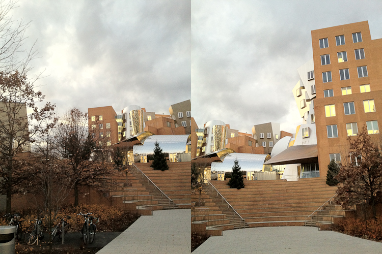
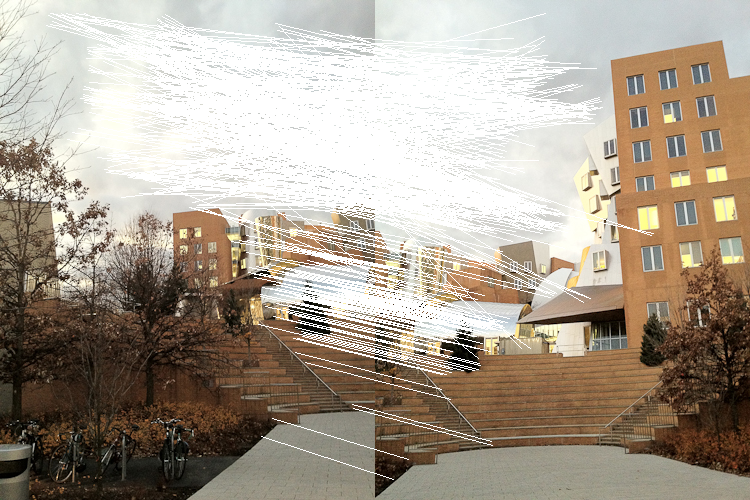
As a set of sample images to use for the stitching exercise, I took two pictures of the Stata Center at MIT. It is home to CSAIL (the Computer Science and Artificial Intelligence Laboratory), where I and many others spend much of our MIT careers in. I really like using it as a case study for image stitching because as you can see, the building is pretty weird, leaving many opportunities for feature detection to go wrong!
img1 = load("imgs/stata-1.png")
img2 = load("imgs/stata-2.png")
[img1 img2]
size(img1)
Extracting Feature Points
The first step to stitching two images together is finding feature points, sometimes called keypoints. The main purpose of feature points are to identify points in an image that are "interesting", for some value of interesting. When we are doing image stitching, we generally think points are interesting if they correspond to "corners" in the image. Basically, points at which boundaries happen between objects. The idea is that if we can identify points at the corners of objects, they are unique enough to match nicely if they appear in another image. Of course, this does not happen in practice, but it works fairly well, as we shall see later on.
One method to finding image corners is the Harris corner method, which uses the Sobel kernel (which I implemented and talked about in my last post) to find areas in the image that have strong gradients.
Thankfully, the Images.jl package we are familiar with implements imcorner:
?imcorner
This is the first time I've come across the Julia method type, so I assumed that I could just pass the function itself (in this case, the harris function):
# construct keypoints
features_1 = imcorner(img1, harris);
But as you can see, it throws an error. Just to confirm, harris is a real Julia function in the Images package:
?harris
So what's the problem? The problem is that in the imcorner function, method is a keyword argument, not a positional argument. How do you know that? Well, the function signature says:
function imcorner(img::AbstractArray; method::Function = harris, args...)
In case you missed it, there is a ; in between the img argument and the method argument. This means that the img argument is a positional argument, and everything after the ; (starting from method), is a keyword argument. The difference is that for a keyword argument, you always have to specify what variable the argument maps to in the function signature, like this:
features_1 = imcorner(img1, method=harris);
In this case, method is a keyword argument and we explicitly have to specify it when calling imcorner.
Now our function calls work just fine! In Julia, positional arguments come before keyword arguments, and keyword arguments cannot be positional arguments. So once you define an argument after a semicolon, it must always be called with a keyword. You can read more about the differences between positional and keyword arguments in the Julia docs.
Visualizing keypoints
Let's see what type gets returned by imcorner and see if we can visualize the features.
summary(features_1)
sizeof(features_1)
You can see that features_1 is a BitArray - this means it is the same as a binary mask the size of our image. A "True" value at a given index means that pixel is a feature, "False" means it is not a feature. The cool thing about BitArrays is that they only store a single bit of information per entry, rather than say an array of booleans, which uses more bits. You can see that this BitArray only takes up 23440 bytes. (aside: there are 8 bits in a byte, so $23440$ bytes $= 23440 \cdot 8 = 1875520$ bits $= 500 \cdot 375$ bits, one bit per entry in the BitArray)
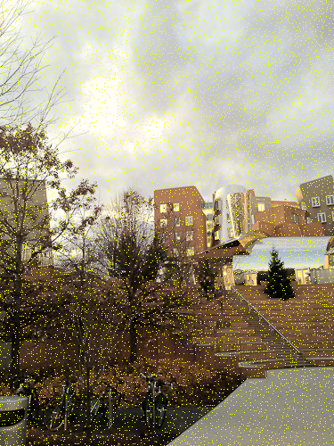
What I want to do is visualize the feature points by drawing a circle around the feature point. I'll do this by iterating over the BitArray and constructing a new one that stores the points that we will turn yellow.
function draw_points(image::AbstractArray, mask::BitArray{2}; c::Colorant=colorant"yellow")
    new_image = copy(image);
    new_image[mask] = c;
    return new_image;
end
draw_points(img1, features_1)
This function works to draw our points, but it is not very generic. The BitArray size is encoded directly. We don't actually care of the BitArray has exactly 2 channels, all we want to know is that it is the same size as the image.
The way we do this is by defining draw_points parametrized by two values T and N. As far as I can tell by reading Julia package code, by convension T is used to represent "Type" and N is used to represent dimension. What this function header says is that for an image of type T with size N, make sure the BitArray mask has the same size. We do this to make sure the calling of the image on the mask doesn't yield an out of bound error.
You'll notice that I also include a color argument as a colorant from the Colors.jl package. Because I specify a default value for this argument, I don't have to call draw_points by passing a color every time. If I don't, it will just use yellow.
function draw_points{T,N}(image::AbstractArray{T,N}, mask::BitArray{N}, c::Colorant=colorant"yellow")
    new_image = copy(image);
    new_image[mask] = c;
    return new_image;
end
draw_points(img1, features_1)
Now let's see if we can use Interact.jl again to visualize the 3 different kinds of corner detectors implemented in ImageFeatures.
using Interact;
@manipulate for m=[harris, shi_tomasi, kitchen_rosenfeld]
    draw_points(img1, imcorner(img1, method=m))
end
As we can see, the differences are pretty minimal, so let's pick Harris corners to use as our keypoint locator and keep exploring parameters. We can see from ImageFeatures that the other way to call imcorner is to specify a percentile and a threshold.
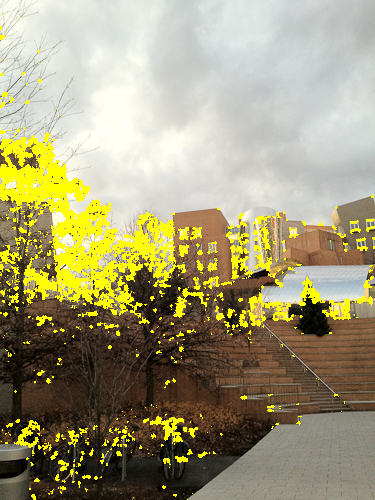
If you specify imcorner WITHOUT these parameters, the function will compute a "local maximum response" of all neighbors, and only return points that have the maximum value of all of its neighbors. If you call imcorner with a percentile, the function does not do mean response and instead returns all the points above the percentile you specified. (Yet another way is to pass a threshold and "false", which just does thresholding without taking percentiles into account, but this is hard to calibrate across methods).
Choosing the local maximum response or the percentile method is one of choice. Usually, local maximum response means you don't have too many feature points that are very close together. This is great for downstream parts of your pipeline, since there are likely to be fewer feature points that look very much alike.
features_1 = imcorner(img1, 0.90, true, method=harris);
summary(features_1)
sizeof(features_1)
One weird quirk of this method is that if you use imcorner and pass arguments, you don't get back a BitArray, but instead an Array of Bool values. Compared to the $23440$ bytes from the BitArray above, this takes $187500 = 500 \cdot 375$ bytes, which is $187500 * 8 = 1500000$ bits, or 8 times more bits.
However, this also means that our implementation for draw_points won't work. We specifically specified that the mask argument had to be a BitArray.
draw_points(img1, imcorner(img1, 0.90, true, method=harris))
What we can do is generalize our function a little bit more. Rather than forcing mask to be a BitArray, we can say that it has to be a type of AbstractArray{Bool, N}, the parent type of both BitArray and Array{Bool}. (Thanks StackOverflow post).
BitArray <: AbstractArray{Bool}
Array{Bool} <: AbstractArray{Bool}
function draw_points{T,N}(image::AbstractArray{T,N}, mask::AbstractArray{Bool, N}, c::Colorant=colorant"yellow")
    new_image = copy(image);
    new_image[mask] = c;
    return new_image;
end
And now we can draw again!
draw_points(img1, imcorner(img1, 0.90, true, method=harris))
Let's see how the percentile affects the Harris corners (I really love Interact!!)
@manipulate for percentile=linspace(0.5, 1.0, 50)
    draw_points(img1, imcorner(img1, percentile, true, method=harris))
end
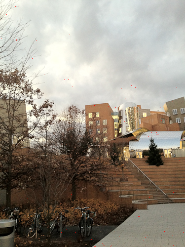
From the outputs, I think we can safely say that the local-max response is the best option for finding feature points of those built into Images.jl - the points are not densely clustered, and we can match them more easily.
Of course, we can combine the two methods, just for kicks:
function corners_percentile_and_local_maximum(img::AbstractArray, percentile)
    percentile_corners = imcorner(img, percentile, true, method=harris)
    corners = falses(size(percentile_corners))
    maxima = map(CartesianIndex{2}, findlocalmaxima(percentile_corners))
    corners[maxima] = true
    return corners
end
@manipulate for percentile=linspace(0.01, 1.0, 50)
    draw_points(img1, corners_percentile_and_local_maximum(img1, percentile), c=colorant"red")
end
As you can see, the resulting corners are very sparse (perhaps too sparse for our needs), so we're just going to stick to the plain old Harris corner detector without playing with percentiles.
Calculating descriptors
Now that we have points on the image that we think are interesting, we want to compute a description of each point that will hopefully help us when trying to find similar points in another image. The purpose of a feature descriptor is to store information about the "orientations" of edges and their magnitudes. The idea is that edges have directionality - a horizontal edge that is darker on the top half is different than a horizontal edge that is darker on the bottom half. So if you are eventually looking to match edges (or corners) from two images together, you need to somehow encode the directionality of these edges in what we call feature descriptors.
There are many options for feature descriptors. You might have heard of SIFT feature points - those work well, except for two problems: (1) the SIFT algorithm is patented, so you can't use it without paying license fees, and (2) SIFT generates a 128-dimensional vector for all the feature points. The good news is that feature descriptors like BRISK, BRIEF, and ORB were created that have similar properties to SIFT while being free and open, and they use fewer bits of information!
The ImageFeatures package provides convenient wrappers around keypoints and features, since this is a pretty common operation in image processing. Of course, this means I'll have to make a new draw_points() method to see my keypoints. But no biggie, it's the same code. Keypoints can be constructed from a BitArray or an Array{Bool}, so we are in the clear.
function draw_points(image::AbstractArray, mask::Keypoints; c::Colorant=colorant"yellow")
    new_image = copy(image);
    new_image[mask] = c;
    return new_image;
end
draw_points(img1, Keypoints(imcorner(img1, method=harris)))
The thing to note is that usually the feature descriptors are calculated a the grayscale version of an image. As it turns out, the information stored in Red, Green, and Blue channels are redundant (self-aside: maybe I'll do an exploratory post on that at some future date), so you really only need to use a single channel that describes all of them to calculate descriptors. Let's say we want to calculate BRISK features on our image. It computes a vector of binary features (i.e. 0s and 1s) that determine whether a particular orientation is present for that keypoint. There's a pretty good graphic on the ImageFeatures.jl docs page about how to visualize the regions used by BRISK features - you can find it here.
ImageFeatures provides an interface for creating a descriptor, but first we need to convert our keypoints to the Feature type so we can store the orientations for each feature point.
?Features
brisk_params = BRISK();
features_1 = Features(Keypoints(imcorner(img1, method=harris)));
desc_1, ret_features_1 = create_descriptor(Gray.(img1), features_1, brisk_params);
Matching keypoints
If we calculate the descriptors for both images, we can use the match_keypoints function to match both images together. What it does (as implemented in ImageFeatures), is match feature points computed on two images using a Hamming Distance function on the feature descriptors, since BRISK features output a set of binary vectors for each keypoint. The Hamming Distance is basically "how many bits different" are two vectors. So the vectors [1, 1, 1] and [0, 0, 0] have a Hamming Distance of 3, while the vectors [1, 1, 1] and [1, 1, 0] have a Hamming Distance of 1. What this means is that the smaller the Hamming distance between two keypoint descriptors, the more likely they are to match. To make sure that only one keypoint in each image is matched, for each keypoint in the first image, take the keypoint in the second image with the smallest Hamming distance.
I'm going to make a wrapper get_descriptors function so I don't need to remember all the arguments to pass.
function get_descriptors(img::AbstractArray)
    brisk_params = BRISK();
    features = Features(Keypoints(imcorner(img, method=harris)));
    desc, ret_features = create_descriptor(Gray.(img), features, brisk_params);
end

function match_points(img1::AbstractArray, img2::AbstractArray, threshold::Float64=0.1)
    desc_1, ret_features_1 = get_descriptors(img1);
    desc_2, ret_features_2 = get_descriptors(img2);
    matches = match_keypoints(Keypoints(ret_features_1), Keypoints(ret_features_2), desc_1, desc_2, threshold);
    return matches;
end
We can then use these matches to draw a line between the matched points from the two images. I'll need to install ImageDraw to make that work, because it implements a line function to draw a line between two points on an image. It is not an official package yet, so we just clone it from Github the same way we did with ImageFeatures.
# Pkg.clone("https://github.com/JuliaImages/ImageDraw.jl");
using ImageDraw;
matches = match_points(img1, img2, 0.1);
function draw_matches(img1, img2, matches)
    grid = [img1 img2];
    offset = CartesianIndex(0, size(img1, 2));
    for m in matches
        line!(grid, m[1], m[2] + offset)
    end
    grid
end
The end result
draw_matches(img1, img2, matches)
You can see that we get some pretty decent results! The sky is problematic, but skies are always going to be problematic, so I'm not too worried. We can probably get rid of that at the filtering and stitching stage in the next post.
However, to do the actual stitching we'll have to use the matched points to compute a transformation from one image to another (known as a homography), while rejecting the bad matches. Then we'll have to actually do the image stitching portions and correct any errors there.
Join me next time when I explore homographies, image transformations, and stitching. I found this package about projective geometry, so maybe I'll take a look at that one!
Final thoughts
Extracting image features is a tricky business, and it is often dependent on the domain, type of image, white balance, etc. Before neural networks became popular, these manual orientation and gradient methods were all the rage. In computational photography and graphics, these methods are still going strong because they yield great results. I would be interested, when I’m more familiar with Julia, to dive into using a neural-network-based approach to extracting and matching keypoints between images. Who knows where my next project will take me!
Thank you for reading, as usual! I would love to hear from you if you have any suggestions, comments, or ideas for what I should learn next.
