
Image Stitching: Part 2
This is Part 2 of 2 in my posts about how to stitch two images together using Julia. It’s rough around the edges, since I’m learning how to do this myself. In Part 1 I talked about finding keypoints, descriptors, and matching two images together. This time, in Part 2, I’ll talk about how to estimate the image transformation and how to actually do the stitching.
Updating Julia versions
For Part 2 of image stitching, I upgraded to Julia 0.6.0. The process was quite painless - download the .tar.gz file from the julialang.org, extract it, and add the bin/ directory from the extracted archive into my path, as I described in my initial post about setting up Julia.
Because I wanted to use the latest versions of some packages (and in Julia, they change often!) I had to do some updates before launching the Jupyter Notebook:
>>> Pkg.update();
>>> using IJulia;
>>> notebook(dir="notebooks/", detached=true);
I also had to make sure to change my Jupyter kernel to Julia 0.6.0 - in the menu bar at the top of the page, click on “Kernel” –> “Change Kernel” –> “Julia 0.6.0”. No reason to stay stuck to old code!
Updating some image drawing functions
One of the packages that I had to image (ImageDraw, used for drawing shapes on images), updated their API for drawing lines. There is no longer a syntactic sugar called line for drawing lines on images; instead, there is a single draw method that accepts targets and Drawable objects. I changed my previous code:
line!(grid, m[1], m[2] + offset)
to
draw!(grid, LineSegment(m[1], m[2] + offset))
And everything worked great.
I’ve included my notebook here. You can see the original on Github if you like.
You can also skip to any of the headers below:
- Calculate Transformation
- Transform Image
- RANSAC: Improving Homography Estimation
- Merging Images
- Conclusion and Summary
In this notebook, I will work on part 2 of the image stitching series. Between this post and the previous post, I go through all 7 steps of an image stitching pipeline:
- Extracting feature points (Part 1)
- Calculate descriptors (Part 1)
- Match points (Part 1)
- Calculate transformation (Part 2)
- Transforming the image (Part 2)
- Using RANSAC to improve transformation computation (Part 2)
- Stitch images (Part 2)
In this notebook, I'll go through Part 2: calculating a transformation and actually stitching the images together. In the course of writing this post, I learned all about OffsetArrays and how they can be useful for image processing in Julia!
using ImageFeatures, Images, FileIO, ImageDraw;
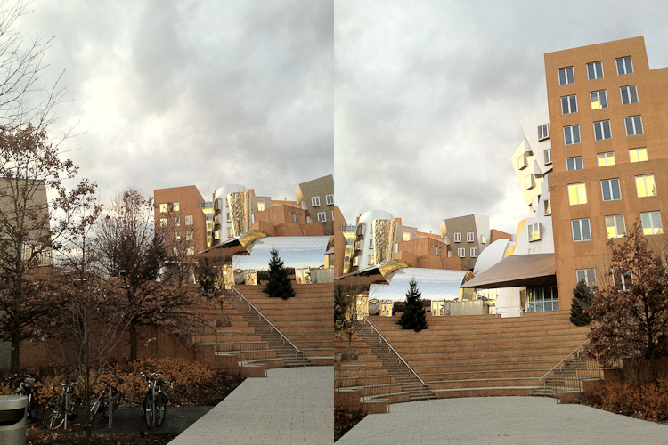
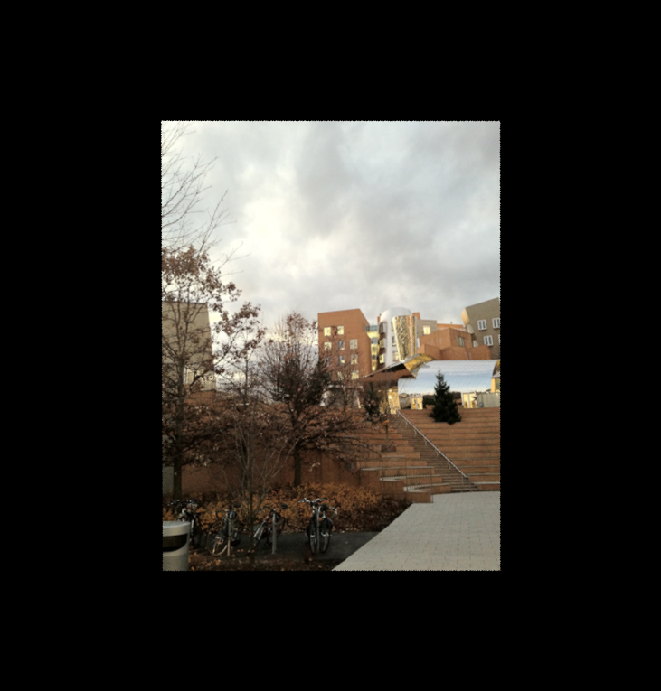
I'll use the same two images I used in the previous post, two images of the Stata Center in Cambridge, MA. At the end of the post, we'll stitch them together in one large image.
img1 = load("imgs/stata-1.png")
img2 = load("imgs/stata-2.png")
[img1 img2]
To recap steps 1 through 3 from the previous post, we extracted feature points, calculated feature descriptors, and matched the points together. I'm going to copy over the get_descriptors and match_points functions directly.
function get_descriptors(img::AbstractArray)
    imgp = parent(img)
    brisk_params = BRISK()
    features = Features(Keypoints(imcorner(imgp, method=harris)))
    desc, ret_features = create_descriptor(Gray.(imgp), features, brisk_params)
end

function match_points(img1::AbstractArray, img2::AbstractArray, threshold::Float64=0.1)
    img1p = parent(img1)
    img2p = parent(img2)
    desc_1, ret_features_1 = get_descriptors(img1p)
    desc_2, ret_features_2 = get_descriptors(img2p)
    matches = match_keypoints(
        Keypoints(ret_features_1), Keypoints(ret_features_2),
        desc_1, desc_2, threshold)
end
But, I'm going to modify my draw_matches functions slightly. It might be the case that we want to match points between two images that are different vertical sizes. To make this happen, we will first need to put both images on the same canvas. To do this, I'm going to make a pad_display function and update my draw_matches function to use it. I in fact figured out that I needed this modification much later in the process of creating this post, but the beauty of Jupyter notebooks is that I can do back and edit things as I need, and use them later.
# this function takes the two images and concatenates them horizontally.
# to horizontally concatenate, both images need to be made the same
# vertical size
function pad_display(img1, img2)
    img1h = length(indices(img1, 1))
    img2h = length(indices(img2, 1))
    mx = max(img1h, img2h);
    hcat(vcat(img1, zeros(RGB{Float64},
                max(0, mx - img1h), length(indices(img1, 2)))),
        vcat(img2, zeros(RGB{Float64},
                max(0, mx - img2h), length(indices(img2, 2)))))
end

function draw_matches(img1, img2, matches)
    # instead of having grid = [img1 img2], we'll use the new
    # pad_display() function
    grid = pad_display(parent(img1), parent(img2));
    offset = CartesianIndex(0, size(img1, 2));
    for m in matches
        draw!(grid, LineSegment(m[1], m[2] + offset))
    end
    grid
end
Let's make sure it all works!
matches = match_points(img1, img2, 0.08);
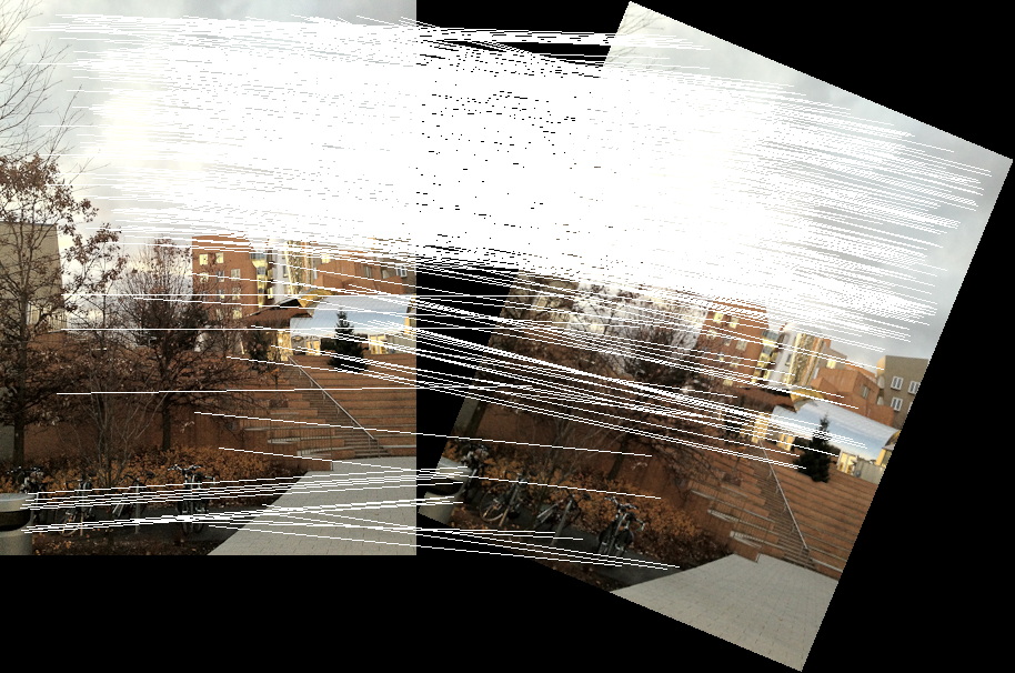
draw_matches(img1, img2, matches)
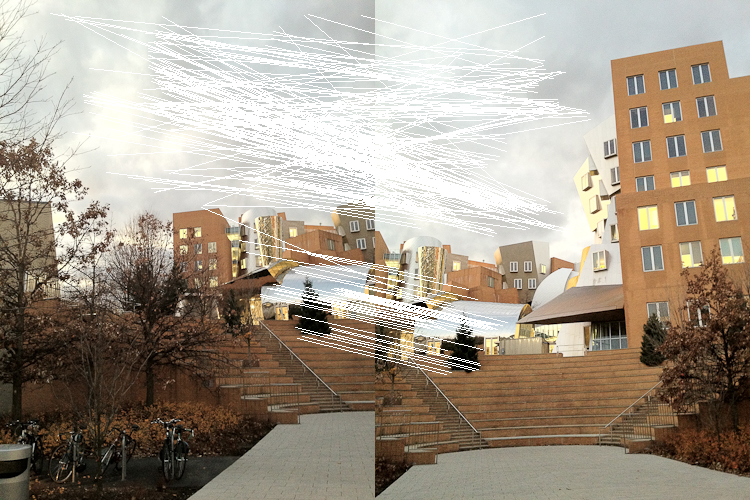
Note that the draw_matches function throws a warning that comes from the ImageDraw package. Right now we're just going to ignore this warning, but hopefully in a future notebook I can figure out how to fix it!
Calculate Transformation
Now that we've found the pairs of pixels that correspond between the two images, we can use those matches to find a matrix that describes the transformation from one image to another. We can then use this transformation to warp one of the images and do the stitching.
To calculate the transformation from one image to another, we compute a transformation called a homography. It is based on the "pinhole camera assumption", where the same scene taken from the same camera is related by rotation, translation, and skew. This OpenCV tutorial has a good, practical example of homography estimation with some geometric examples.
A homography matrix has 8 free parameters - this means that with 4 pairs of matched points in our image, we can compute a homography that describes how to transform from the first set to the second set of points.
Usually, I am a fan of reusing someone else's code that is well-written, but in this case I had to take matters into my own hands.
The ImageProjectiveGeometry package implements a homography filling algorithm, but the package was built for Julia 0.4 and I had a hard time getting to play nice with my Julia 0.6 environment. Instead, I am going to write my own code for this in Julia.
My homography function is going to take some matches returned from our descriptor matching function; as a reminder, matches is returned as an array of Keypoints.
To make our homography computation easier, we will create a new type (with the immutable keyword) that is a 3 x 3 matrix, that is also a subtype of an AbstractAffineMap from the CoordinateTransformations package. We do this because the CoordinateTransformations package has a warp function that can be used to apply this transformation (i.e. homography) to images, without having to write our own projection code.
using CoordinateTransformations, StaticArrays, ImageTransformations;
immutable Homography{T} <: AbstractAffineMap
    m::SMatrix{3, 3, T, 9}
end

# having T in the RHS forces calling the constructor again
Homography{T}(m::AbstractMatrix{T}) = Homography{T}(m);
Now that we've set up the homography data type, we can actually write the function that will compute the homography. We want to apply it to an array if Keypoints that we previously computed (and matched).
There are typically 2 ways in which a homography is computed:
- "Exactly", using 4 pairs of points. Because there are 9 unknowns in the homography matrix (one of which we always set to 1, so it's really 9 up to a scale factor), we can solve an exact system of linear equations with 4 pairs of points to get the exact homography between the pairs. Each pair of points creates 2 linear equations, so with 4 pairs of points you get 8 equations, which is enough to determine an exact solution (up to a scale factor, since we want the bottom-right entry in the homography matrix to be 1).
- Using the "least-squares" method. With more than 4 pairs of points, your system equations is overconstrained, so you need to find the best "average" homography that fits all the pairs.
To set up the system of equations to compute a homography, we set up a a system of equations as follows: knowing that a homography relates two points $u$ and $v$ in 3D space by $v = H u \rightarrow H u - v = 0$, which is homogenous linear equation of the form $A x = 0$ (with some clever re-arranging of the coefficients). Because we deal with 2D points (i.e. locations in an image), the 3rd dimension of $u$ and $v$ is always 1. With a little bit of algebraic manipulation you get that each pair of points contributes these 2 equations to the matrix $A$:
\begin{equation} H u - v = 0 \end{equation}\begin{equation} \begin{bmatrix} h_1 & h_2 & h_3 \\ h_4 & h_5 & h_6 \\ h_7 & h_8 & h_9 \end{bmatrix}\begin{bmatrix} u_1 \\ u_2 \\ 1 \end{bmatrix} - \begin{bmatrix} v_1 \\ v_2 \\ 1 \end{bmatrix} = 0 \end{equation}\begin{equation} \begin{bmatrix} 0 & 0 & 0 & -u_1 & -u_2 & 1 & v_2 u_1 & v_2 u_2 & v_2 \\ u_1 & u_2 & 1 & 0 & 0 & 0 & -v_1 u_1 & -v_1 u_2 & -v_1 \end{bmatrix}\begin{bmatrix} h_1 \\ h_2 \\ h_3 \\ h_4 \\ h_5 \\ h_6 \\ h_7 \\ h_8 \\ h_9 \end{bmatrix} = 0 \end{equation}\begin{equation} A x = 0 \end{equation}When we have more points, we just have more instances of the pair of equations on the left-hand side in Equation (3), with the same homography-matrix-as-a-column-vector on the right.
The good news is that in both cases (exact solution & least-squares estimation), we can use the same method: applying singular value decomposition (SVD) on the resulting equation matrix $A$ and take the smallest eigenvector. When do this with only 4 points, you get the exact solution to the system of equations.
My compute_homography function below re-creates this linear system of equations and solves it using SVD.
function compute_homography(matches::Array{Keypoints})
    # eigenvector of A^T A with the smallest eigenvalue

    # construct A matrix
    A = zeros(2 * length(matches), 9)
    for (index, match) in enumerate(matches)
        match1, match2 = match
        base_index_x = index * 2 - 1
        base_index_y = 1:3
        A[base_index_x, base_index_y] = float([match1.I...; 1;])
        A[base_index_x + 1, 4:6] = A[base_index_x, base_index_y]
        A[base_index_x, 7:9] =
            -1.0 * A[base_index_x, base_index_y] * match2.I[1]
        A[base_index_x + 1, 7:9] =
            -1.0 * A[base_index_x, base_index_y] * match2.I[2]
    end

    A
    # find the smallest eigenvector, normalize, and reshape
    U, S, Vt = svd(A)

    # normalize the homography at the end, since we know the (3, 3)
    # entry should be 1.
    Homography(reshape(Vt[:, end] ./ Vt[end][end], (3, 3))')
end
As an aside, I learned about multi-line commands in Julia. Take for instance line 12 in the compute_homography function above. It was too long to read on the blog, so I split it up into multiple lines. Julia will ignore all whitespace (and look at the next line for command input) until it finds a complete command. So you can put any whitespace you want in your Julia code. I like to keep it ~80 characters per line, for easy readability.
Now that we've computed the homography, we want to actually apply it to points that we got from the image.
Because a homography is a 3x3 matrix, it is applied to a point in 3D space. However, if we want to apply it to a point in 2D space (like for example, the point $(1, 1)$, which is the image origin), we need to append $1.0$ as the last element.
The output of a homography transformation is always a point in 2D space, so we need to transform the result of the homography from a 3D coordinate to a normalized 2D coordinate. We take advantage of Julia's multiple dispatch (i.e. calling of methods based on the types of the arguments) to make a bunch of utility methods that override the () operator and take care of this 3D / 2D conversion for us.
# these 5 functions override the () operator, so we can
# do something like H(image) and have H (the homography)
# be applied to the image, SVector{2}, cartesian index,
# or tuple.
function (trans::Homography{M}){M}(x::SVector{3})
    out = trans.m * x;
    out = out / out[end];
    SVector{2}(out[1:2])
end

function (trans::Homography{M}){M}(x::SVector{2})
    trans(SVector{3}([x[1], x[2], 1.0]))
end

function (trans::Homography{M}){M}(x::CartesianIndex{2})
    trans(SVector{3}([collect(x.I); 1]))
end

function (trans::Homography{M}){M}(x::Tuple{Int, Int})
    trans(CartesianIndex{2}(x))
end

function (trans::Homography{M}){M}(x::Array{CartesianIndex{2}, 1})
    CartesianIndex{2}.([tuple(y...) for y in trunc.(Int, collect.(trans.(x)))])
end

# we need to override the inverse function on our homography
function Base.inv(trans::Homography)
    i = inv(trans.m);
    Homography(i ./ i[end])
end
Let's test our homography function (and the displaying of the result) on a simple transformation we apply on our "wild" test images from above.
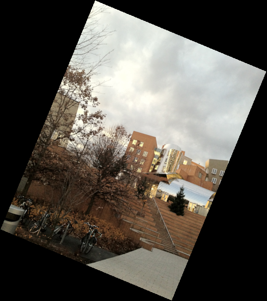
Using the CoordinateTransformations package, let's rotate one of our images a little it. Because we know the absolute transformation (a rotation), we can write it in terms of a homography and test that our compute_homography function works as expected.
rotation = LinearMap(RotMatrix(pi/8));
img1rot = warp(img1, rotation)
Transform Image
Now that we have a homography (transformation) matrix, we need to apply the homography to each pixel in the first image. This will assign a new location to each pixel, effectively warping the original image into the same "space" as the second image.
A homography transforms an image into a new space. The inverse (i.e. the matrix inverse) of the homography transforms the transformed image back into the original image. To see what that's like, let's warp the rotated image by the inverse of the rotation.
out = warp(img1rot, inv(rotation))
The type of the output image is an OffsetArray - a type that we'll look at later.
typeof(out)
Let's use this simple rotated image to test our maching and homography computation code by computing the homography, drawing the two images side by side, and drawing the point matches. In the ideal case, we want the computed homography from our compute_homography function to exactly find the rotation.
The first step is to find the matches between the image and the rotated image.
matches_rot = match_points(img1, img1rot, 0.07);
Let's visualize all the matches we got and see what happens:
draw_matches(img1, img1rot, matches_rot)
Looks great! We seem to have matched the points in this image pretty nicely (except for whatever happens with the sky). Let's see if we get the same luck with our computed homography!
H_computed_rot = compute_homography(matches_rot)
We can see that the computed homography matrix looks unintuitively strange (it doesn't look like a rotation matrix, if you're used to manipulating those). So instead we will just apply our homography to our image and draw matches between them to visualize.
warp(img1rot, H_computed_rot)
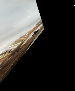
Oops, that doesn't look great! Let's finish the last step of homography computation to make this more robust!
RANSAC: Improving Homography Estimation
The homography computation is a linear estimator. Like all linear estimators, it is not robust to outliers. We got such a bad image above because some of the matches (mostly in the sky) because there were a number of matches that are outliers.
The RANSAC (RANdom SAmple Consensus) method of homography estimation was invented to reduce the effect of outliers on the homography computation. The idea is simple: we can compute an exact homography using four random matched points, and see how well those points fit the other matches. The points that fit the matches well are called inliners (as opposed to outliers). Keep doing this for a number of iterations: one of the homographies that fits the point the best (i.e. had those most inliers). Take ALL those points, and recompute a least-squares homography using all those inliers.
Let's get to it!
function apply_ransac(matches, n_iters=20, eps=20)
    best_homography_inliers = []
    best_num_inliers = 0

    # for N times, use 8 points to estimate the homography
    for i in 1:n_iters
        # randomly pick 4 points from matches
        matches_sub = rand(matches, 4)

        # calculate the homography
        H_sub = compute_homography(matches_sub)

        # calculate the number of inliers.
        # apply the homography to all the points
        # in the first image. calculate descriptors.
        img1_points = [m[1] for m in matches]
        img2_points = [m[2] for m in matches]
        out = H_sub(img1_points)
        dists = [sqrt(x.I[1]^2 + x.I[2]^2) for x in (out - img2_points)]

        # if diff < epsilon, its an inliner
        inliner_indices = dists .< eps
        num_inliers = sum(inliner_indices)

        # if this is the best we got so far, store it
        # and all the inliers
        if num_inliers > best_num_inliers
            best_homography_inliers = matches[inliner_indices]
            best_num_inliers = num_inliers
        end
    end

    # calculate the new homography with all the inliers
    H = compute_homography(best_homography_inliers)
end
Now that we have the RANSAC method, we just need to apply it. We've picked an arbitrary number of iterations to make sure we have enough chances to find the right combination of points. Picking the right number of iterations is a bit of a tricky thing, but more is (usually) never worse. Let's go with a few hundred and see where that leaves us.
H_ransac_rot = apply_ransac(matches_rot, 500)
Now that looks more like a rotation matrix! Let's take a look!
warp(img1rot, H_ransac_rot)
Bam!
Let's see how far we get when we apply what we have so far to the original two images:
matches = match_points(img1, img2, 0.08)
H_ransac = apply_ransac(matches, 500)
new_img = warp(img2, H_ransac)
Yay! Our homography computation worked! Now, the last step is to merge the images together into a single canvas.
Merging Images
Now that we have the right transformation (and it looks ok), the last step to stitching the images together in the same canvas.
The idea goes like this: both images we want to merge originally came from the same "coordinate system." A homography describes the geometric relationship between the two images, and that includes translation. So, all we need to do is figure out the translation between the first and second images, create a new image that contains both, and put the pixels from both images into that same canvas.
Now this is where Julia really shines. Remember how the warped image from above is an OffsetArray? Like this:
typeof(new_img)
We will use this to our advantage when merging images. OffsetArrays are basically arrays, but with arbitrary start and stop indices. So while a "standard" image starts at (0,0) and goes to (1280,720) or something similar, an OffsetArray has the same height and width but might start at (-10, -100).
So how we'll use this is as follows: our new merged image canvas will be an OffsetArray. The sizes will be determined by the two images we want to merge (one is an AbstractArray, or "regular image" and one is an OffsetArray, or "warped image").
As an aside, I figured out that to find the "offsets" of an OffsetArray you use .start and .stop on the axes().val object.
Once we have the dimensions of this new offset array, we are just going to put the original image into it starting at coordinate (1, 1) and ending at the size of the image.
For the merged image, we need to do something a bit more nuanced: because we projected the image into a new space, the places were there was no original pixel from the image became black. In our merging code, we want to ignore these pixels, and only place the non-black pixels into the new canvas. So we iterate through all the pixels (using indices() as an iterator, like suggested in the Julia docs about OffsetArrays, and ignore any black pixels.
Once we're one, our resultant new, merged image is an OffsetArray that is exactly an image!
using OffsetArrays
function merge_images(img1, new_img)
    axis1_size =
        max(axes(new_img)[1].val.stop, size(img1, 1)) -
        min(axes(new_img)[1].val.start, 1) + 1
    axis2_size =
        max(axes(new_img)[2].val.stop, size(img1, 2)) -
        min(axes(new_img)[2].val.start, 1) + 1

    # our new image is an offset array
    combined_image = OffsetArray(
        zeros(RGB{N0f8}, axis1_size, axis2_size), (
            min(0, axes(new_img)[1].val.start),
            min(0, axes(new_img)[2].val.start)))

    # we just put the image directly into the new combined canvas
    combined_image[1:size(img1, 1), 1:size(img1, 2)] = img1

    # merge all the pixels into the new image that are not black
    for i in indices(new_img, 1)
        for j in indices(new_img, 2)
            if new_img[i, j] != colorant"black"
                combined_image[i, j] = new_img[i, j]
            end
        end
    end
    combined_image
end
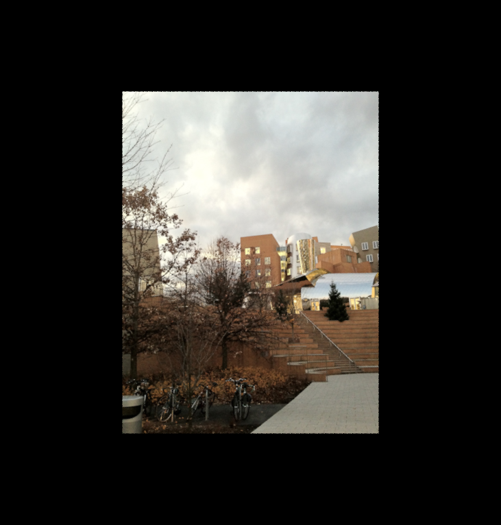
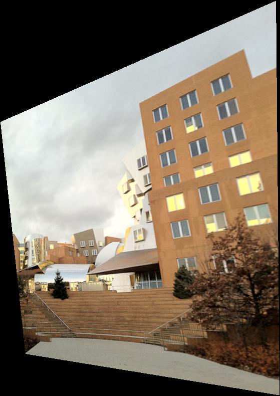
merge_images(img1, new_img)
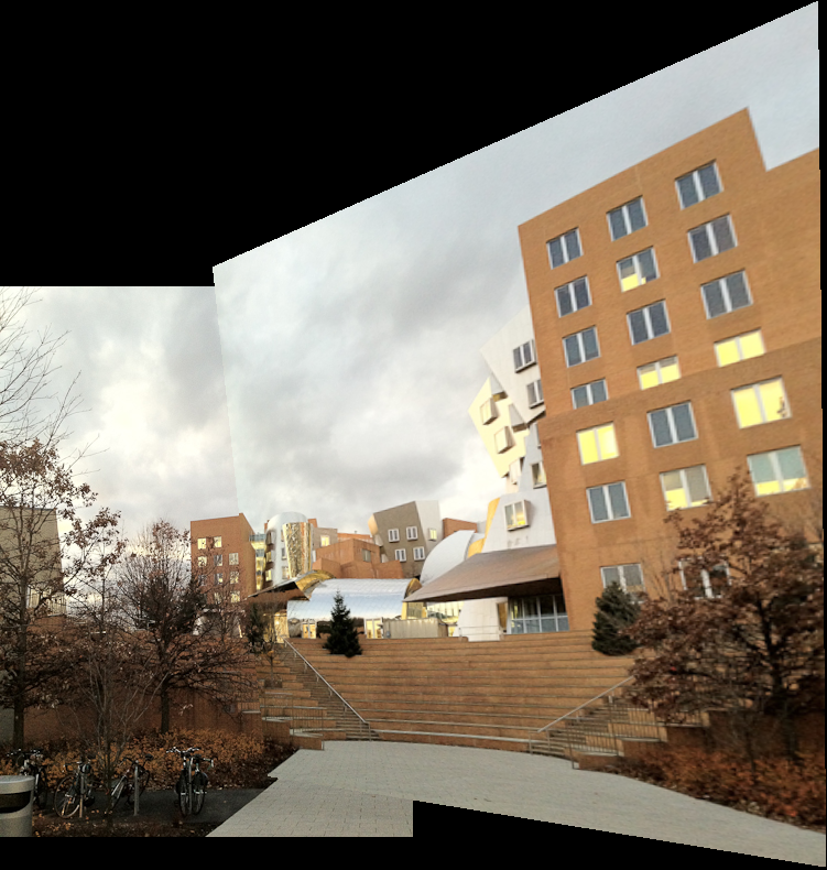
Voila!
Conclusion and Summary
Figuring out how to do panomara stitching in Julia was a LOT of fun. It also took me a while, since I had to learn a bunch of new packages and new concepts. But, all together, stiching two images together in Julia is fairly straightforward, and we generate a merged image in the process.
In this investigation I learned a few things:
- How
OffsetArrayscan make merging images insanely easy! (the corresponding code in C++ is complicated because it involves manually finding the size of the new image together with the offsets) - How multiple dispatch can make applying a homography really easy
- How
StaticArraysandCoordinateTransformationsmake it easy to apply transformations to images.
The caveat is that I did all of this using Julia 0.6. At the time of this writing, some JuliaImages packages weren't ready for 0.7 and above, but hopefully that will change soon.
I hope someone else learning Julia will find my investigations useful. Thanks for reading, and stay tuned for more!
Final thoughts
This notebook was a long time coming (almost a year between parts 1 and 2!) but I’m glad I finally did it. It was tons of fun, and in a future notebook I want to do automatic panorama stitching with multiple images instead of just two! Hopefully this will be equally painless. I am sold on using Julia for image processing - lightning fast, easy to prototype, and easy to get things done!
Thank you for reading, as usual! I would love to hear from you if you have any suggestions, comments, or ideas for what I should learn next.
Here are the ideas I already have:
- Explore more sophisticated methods of image stitching (for example, mean pixel value across multiple pixels, bilaterial filtering, edge smoothing)
- Learning how to fix the warning I see from the
ImageDrawpackage - Multiple-image panorama stitching (instead of just two images)
- Your idea here!